SparseOpt: Why Normalization Hurts Sparse Training (And How to Fix It)
Normalization layers are ubiquitous in modern deep networks — but we show they can skew gradients in sparse layers, causing slow convergence in Dynamic Sparse Training. We identify this problem analytically and propose a simple sparsity-aware optimizer to fix it.
TL;DR
Dynamic Sparse Training (DST) methods like RigL
- BN amplifies gradients non-uniformly in sparse layers. Because neurons in a sparse layer have heterogeneous fan-in (different numbers of incoming connections), BN’s normalization scale varies per neuron. This amplifies the gradient of neuron $i$ by a factor of $(1 - s_i)^{-1/2}$, where $s_i$ is the neuron’s sparsity. This skews (rotates and scales) the overall gradient direction.
- DST mask updates make this worse. Every time the sparse mask is updated during training, neuron-wise sparsities change abruptly, causing discontinuous jumps in gradient direction. This destabilizes training and slows convergence.
- SparseOpt fixes the skew with a simple diagonal preconditioner. By rescaling each neuron’s gradient by $\sqrt{1 - s_i}$, the BN-induced distortion is corrected. This can be wrapped around any existing optimizer (SGD, HAM, etc.) with minimal computational overhead.
- Consistent improvements across architectures and datasets. On ResNet50/ImageNet and ResNet20/CIFAR-100, SparseOpt achieves higher accuracy than the baseline under the same training budget, with the largest gains at higher sparsity levels.
The Convergence Problem in Sparse Training
Modern deep networks are growing rapidly in size, making efficiency at training and inference time increasingly important. Sparse neural networks, which use sparse matrices instead of dense matrices, offer a compelling path to reduced computation, especially through Dynamic Sparse Training (DST), which learns sparse topologies directly during training without any dense pretraining
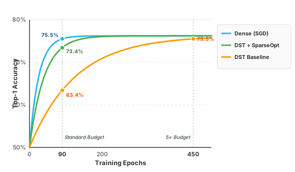
Despite this promise, DST has a well-known weakness: it converges much more slowly than dense training, often requiring as many as five times more epochs to reach the same accuracy
A natural question is: why does DST converge so slowly? Prior work has focused on sparse topology exploration, gradient flow, and initialization
Batch Normalization in Dense Layers: A Quick Recap
Batch Normalization
The standard deviation $\sigma_i$ plays a key role in the backward pass too. Applying the chain rule to the BN equations, the gradient with respect to the pre-activation $x_i^{(b)}$ is scaled inversely by the standard deviation:
\[\frac{\partial L}{\partial x_i^{(b)}} = \frac{1}{\sigma_i} \cdot C_i^{(b)}\]where $C_i^{(b)}$ is a correction term that depends only on the normalized pre-activations and their gradients. In a fully-connected dense layer where every neuron has the same fan-in, all neurons share the same $\sigma_i$ — so BN scales all gradients uniformly, and everything is well-behaved.
The Problem: Heterogeneous Fan-in in Sparse Layers
In a sparse layer, neurons do not all have the same number of incoming connections. Neuron $i$ may have far fewer active weights than neuron $j$. This difference in active connections is known as heterogeneous fan-in.
Specifically, let $s_i \in [0, 1)$ denote the sparsity of neuron $i$ — the fraction of its incoming connections that are zero. If we assume the weights and incoming activations are independent, zero-mean random variables, the pre-activation variance is scaled by its number of active inputs:
\[\text{Var}[x_i'^{(b)}] = (1 - s_i) \cdot \text{Var}[x_i^{(b)}]\]which means its BN normalization scale is:
\[\sigma_i' = \sqrt{1 - s_i} \cdot \sigma_i.\]This difference in scale propagates into the backward pass. Substituting into the BN gradient equations, the gradient with respect to the sparse neuron’s pre-activation is amplified compared to the equivalent dense neuron:
\[\frac{\partial L}{\partial x_i'} = \frac{1}{\sqrt{1 - s_i}} \cdot \frac{\partial L}{\partial x_i}.\]In other words, BN amplifies the gradient of sparse neurons by a factor of $(1-s_i)^{-1/2}$. At 90% sparsity this is a factor of $\approx 3.2\times$; at 95% sparsity it is $\approx 4.5\times$; at 97% sparsity it is $\approx 5.8\times$.
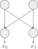
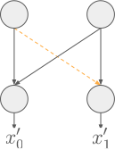
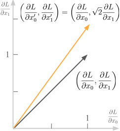
Because different neurons in the same layer will generally have different sparsities $s_i$, these amplification factors are non-uniform across neurons. This non-uniform scaling changes the relative magnitude of different gradient components, thereby rotating the gradient direction — not just its overall magnitude (Figure 2c). The optimizer is no longer descending in the true loss gradient direction; it is descending along a skewed version of it.
Empirical Confirmation
We validated this theoretical prediction empirically using a two-layer MLP on MNIST, measuring the ratio of sparse to dense gradients across a range of sparsity levels.
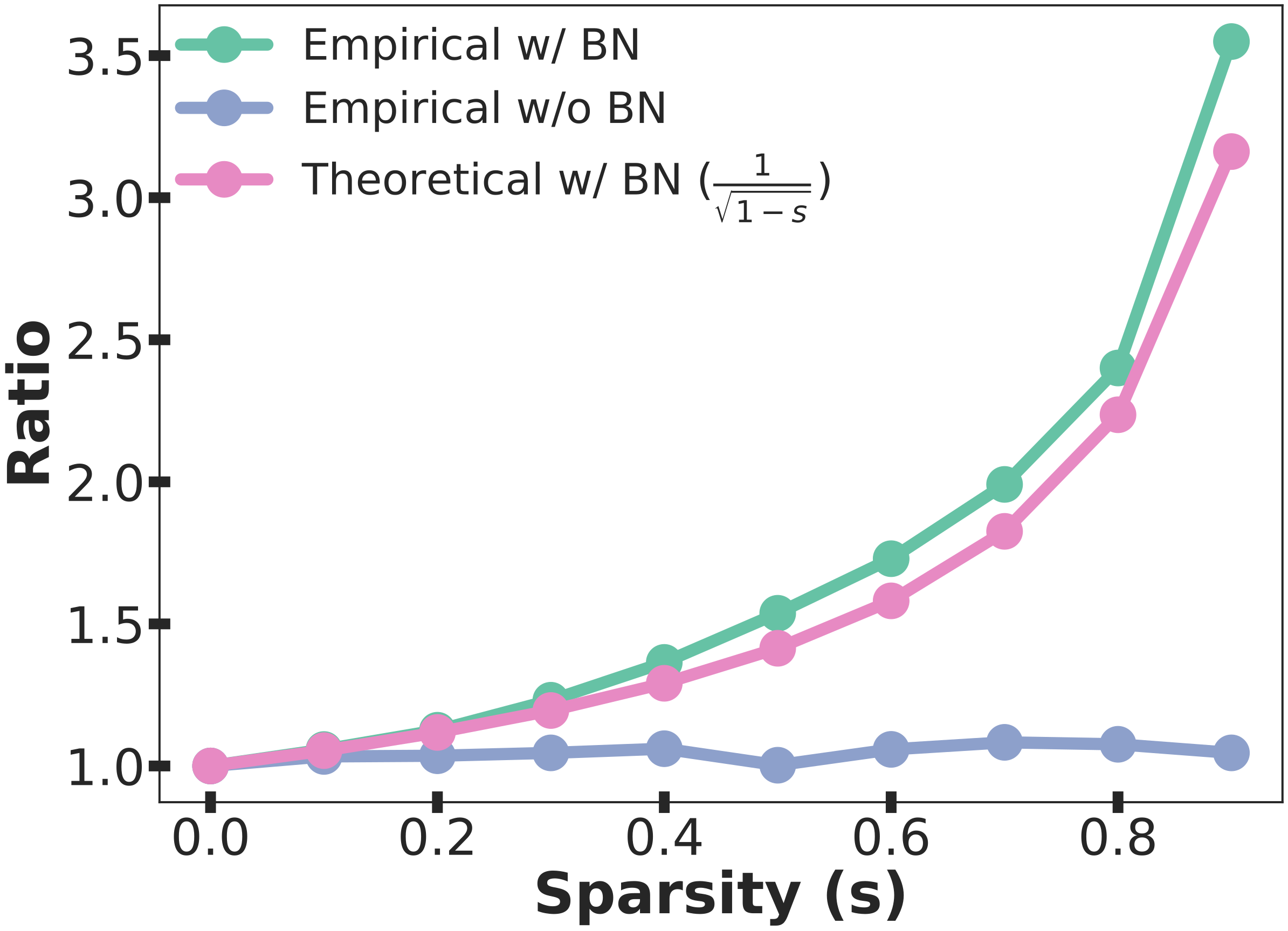
The results (Figure 3) match the theoretical curve $1/\sqrt{1-s}$ closely when BN is present, while gradients remain near a ratio of 1.0 without BN.
Why DST Makes It Worse: Mask Updates and Gradient Direction Jumps
In standard (static) sparse training, the sparse mask is fixed throughout training. While BN-induced gradient skew still occurs, the neuron-wise sparsities ${s_i}$ remain constant, so the skew is at least consistent.
In Dynamic Sparse Training, the mask is updated periodically — every $\Delta T$ training steps — by pruning some connections (e.g., by weight magnitude) and regrowing others (e.g., by gradient magnitude in RigL
Since BN rescales gradients by $(1 - s_i)^{-1/2}$, every mask update triggers an abrupt, neuron-dependent change in gradient scaling. The optimizer suddenly finds itself descending in a different direction — not because the loss landscape changed, but because the normalization-induced distortion changed. This introduces recurring optimization noise at each mask update, exacerbating training instability and slowing convergence.
To the best of our knowledge, this is the first work to identify Batch Normalization as a source of training instability in DST and sparse training more broadly.
SparseOpt: A Sparsity-Aware Preconditioned Optimizer
The source of the problem is clear: BN introduces a neuron-dependent gradient scaling factor of $(1 - s_i)^{-1/2}$. The fix is equally clear: cancel this factor by rescaling each neuron’s gradient by the inverse, $\sqrt{1 - s_i}$.
Formally, for a weight matrix $W$, the column $W[:, i]$ corresponds to all incoming weights of neuron $i$. We apply a diagonal preconditioner $D$ where the entry corresponding to neuron $i$ is $\sqrt{1 - s_i}$. To approximately preserve the overall gradient norm, we also normalize by $\sqrt{1 - s_{\text{avg}}}$, where $s_{\text{avg}}$ is the average neuron sparsity across the layer.
The resulting SparseOpt update rule is:
\[w^{t+1} = w^t - \frac{\eta}{\sqrt{1 - s_{\text{avg}}}} D \nabla \mathcal{L}(w^t),\]where $\eta$ is the learning rate. This can be understood as a diagonal preconditioning step that corrects the BN-induced gradient imbalance while approximately preserving the global gradient norm.
Note for dense layers: When all neurons have the same sparsity $s_i = 0$, we have $\sqrt{1 - s_i} = 1$ for all $i$, so $D = I$ and the update reduces exactly to standard SGD. Dense training is a special case of our formulation.
How to Apply SparseOpt
SparseOpt is straightforward to implement. At each training step, after computing gradients:
- For each sparse layer, compute the per-neuron sparsity $s_i = 1 - \text{fan-in}i / N{\ell-1}$.
- Scale each neuron’s incoming weight gradients by $\sqrt{1 - s_i}$.
- Normalize by $\sqrt{1 - s_{\text{avg}}}$ to preserve overall gradient magnitude.
- Pass the corrected gradients to any underlying optimizer (SGD, Adam, HAM, etc.).
The overhead is minimal — it only requires computing sparsity statistics (which are already tracked in DST methods) and a per-neuron scalar multiply.
Experimental Results
We validate SparseOpt on two standard benchmarks for sparse training:
- ResNet50 / ImageNet with RigL and SET at sparsities $s \in {0.90, 0.95, 0.97}$, with training schedules of 90, 180, and 270 epochs.
- ResNet20 / CIFAR-100 with RigL and SET at the same sparsities, with training schedules of 100, 200, 300, and 500 epochs.
Faster Convergence on ImageNet
We show the ImageNet training and test trajectories for RigL across our evaluation configurations below.
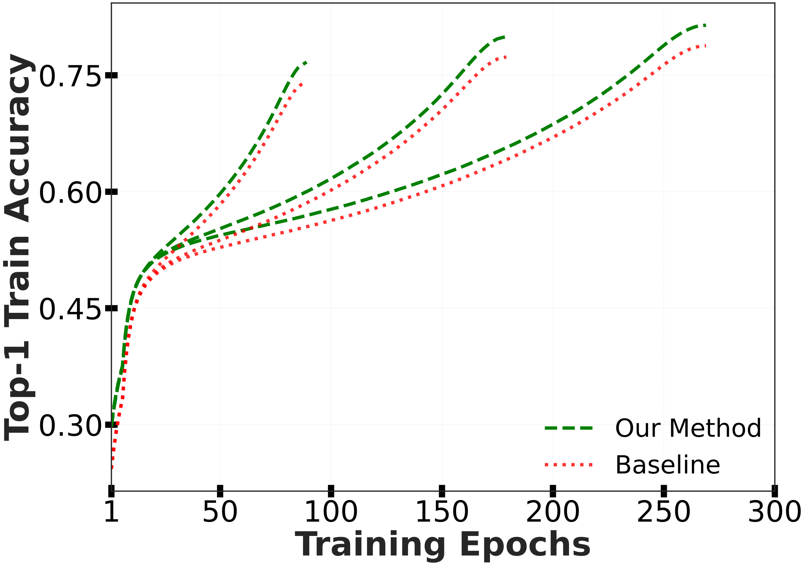
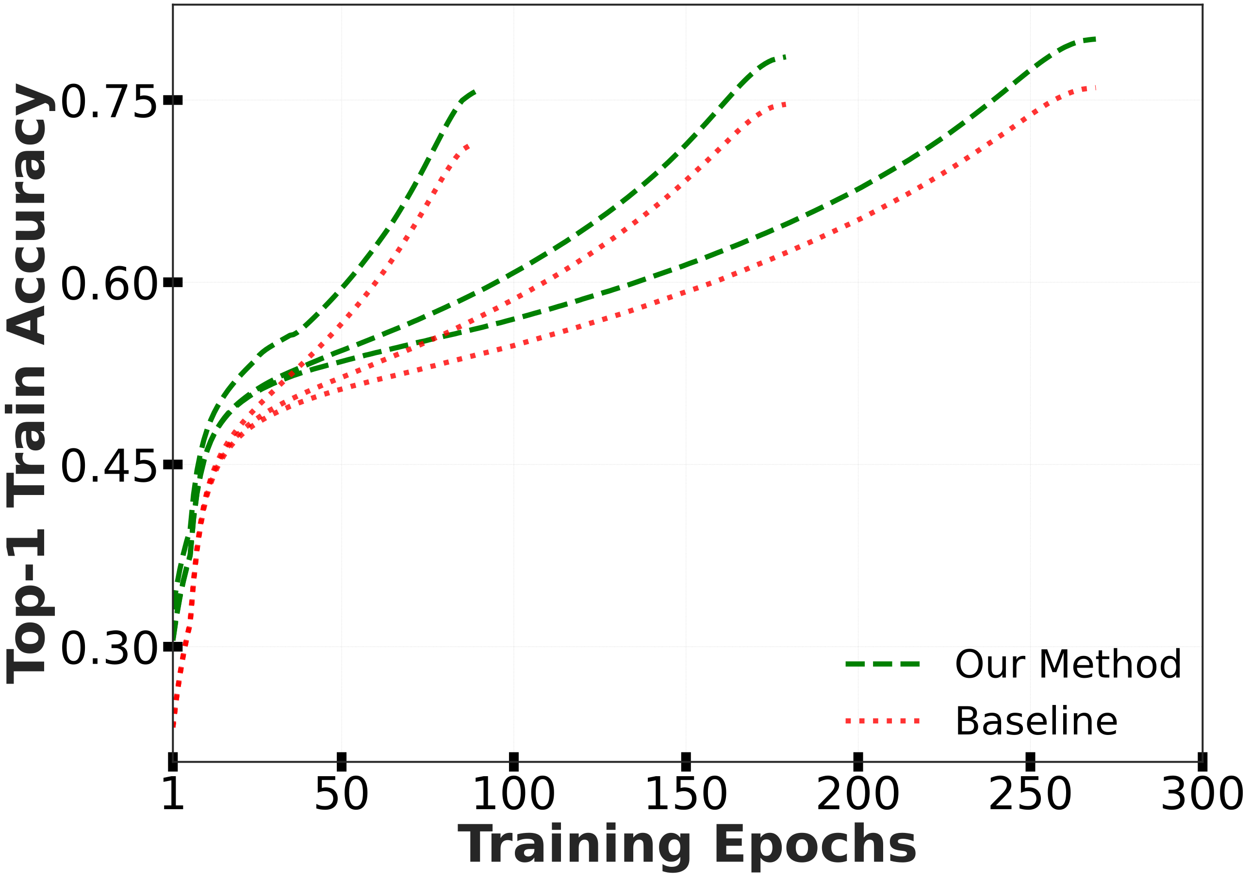
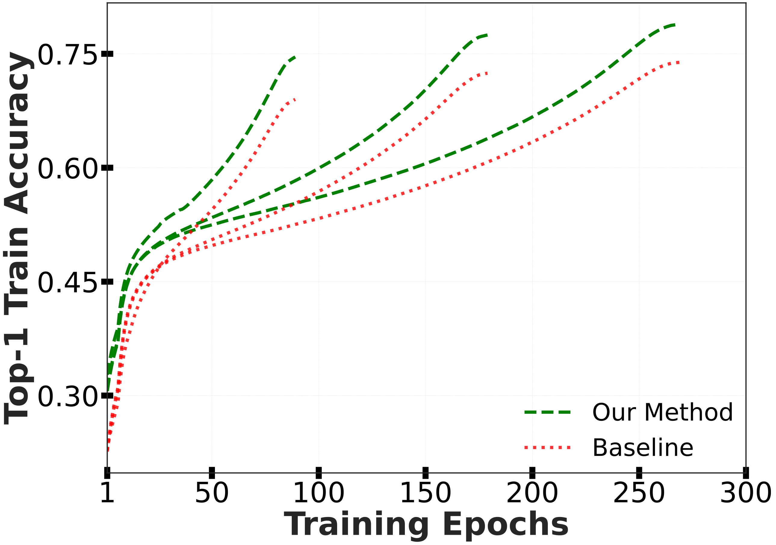
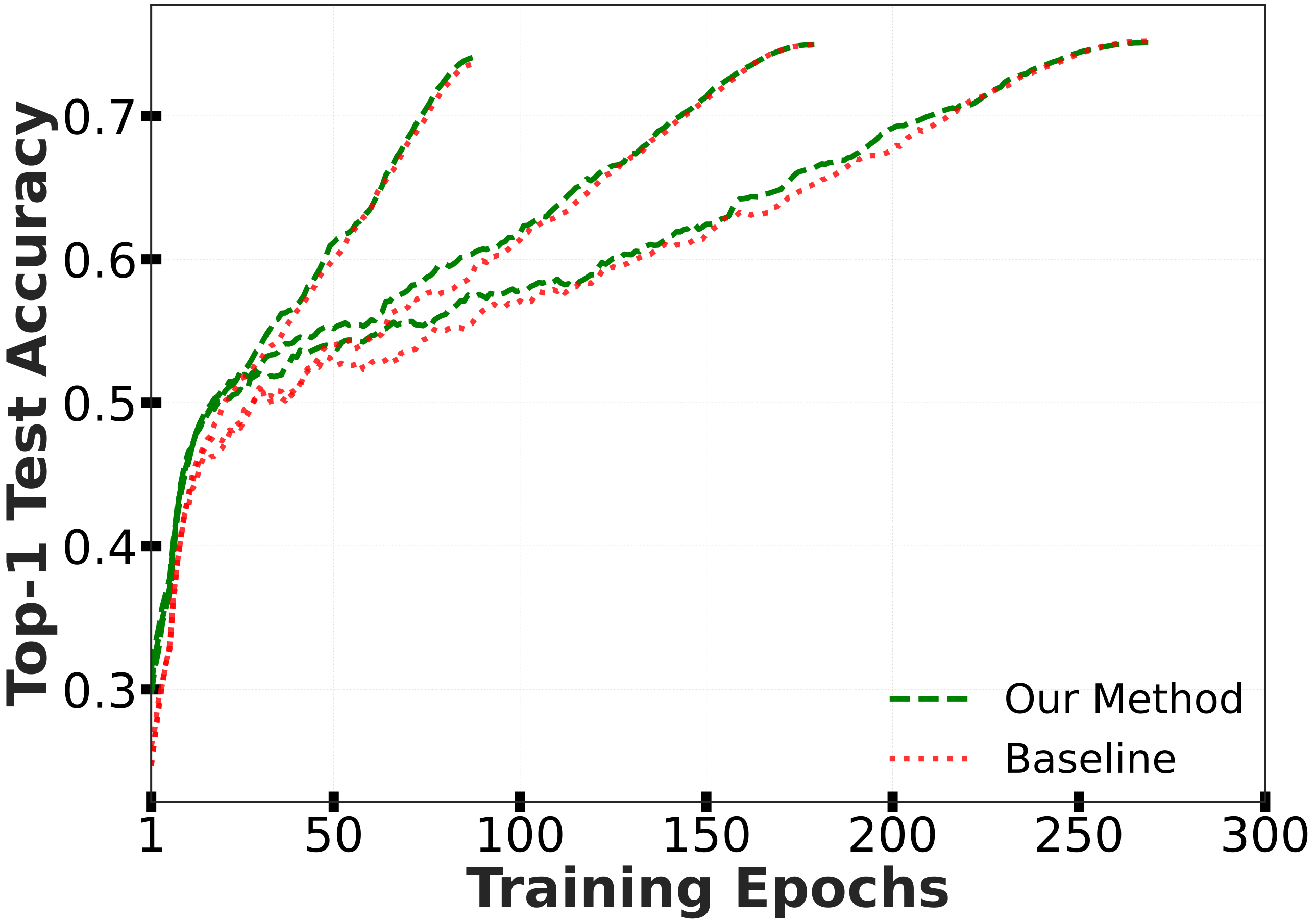
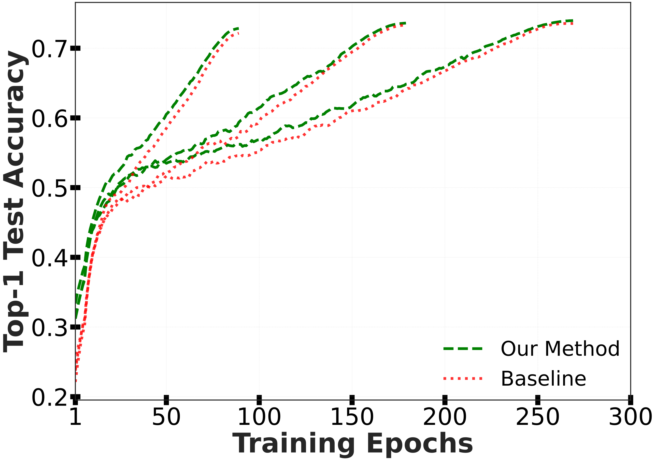
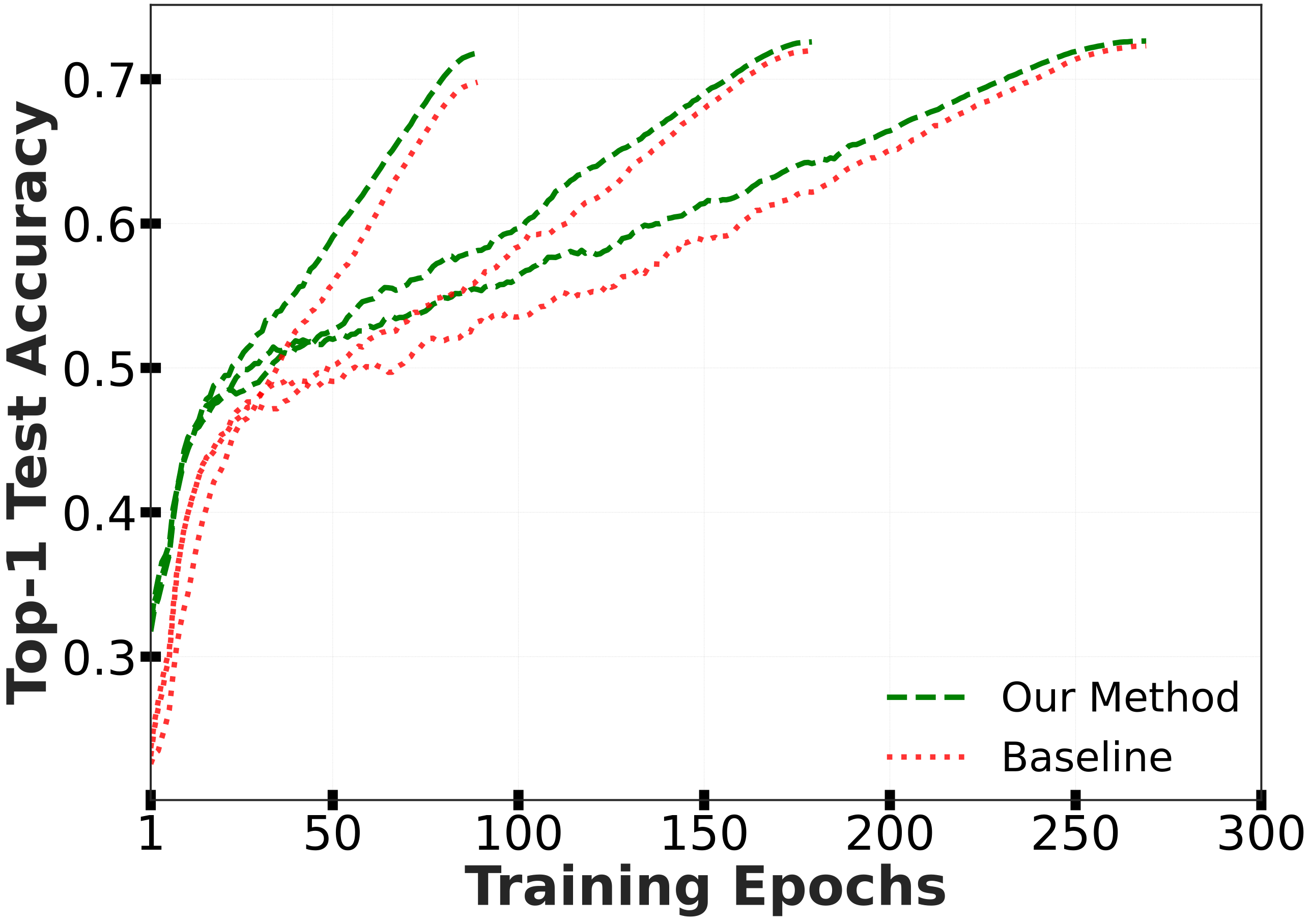
The quantitative results on ImageNet / ResNet50 are shown in the table below. SparseOpt consistently outperforms the baseline across all sparsity levels and training schedules, with the largest gains at 97% sparsity and the shortest training budgets.
| Sparsity | Method | DST | 90 epochs | 180 epochs | 270 epochs |
|---|---|---|---|---|---|
| 90% | Ours | RigL | 74.41 | 75.06 | 75.26 |
| Baseline | RigL | 73.88 | 74.99 | 75.26 | |
| Ours | SET | 74.15 | 74.81 | 74.85 | |
| Baseline | SET | 73.69 | 74.83 | 75.17 | |
| 95% | Ours | RigL | 72.93 | 73.62 | 73.95 |
| Baseline | RigL | 72.33 | 73.36 | 73.62 | |
| Ours | SET | 72.59 | 73.75 | 73.79 | |
| Baseline | SET | 71.84 | 73.51 | 73.82 | |
| 97% | Ours | RigL | 71.15 | 72.65 | 72.66 |
| Baseline | RigL | 69.94 | 72.00 | 72.35 | |
| Ours | SET | 71.43 | 72.40 | 72.73 | |
| Baseline | SET | 70.12 | 72.17 | 72.65 |
Consistent Gains on CIFAR-100
Similar improvements hold on CIFAR-100 / ResNet20 with both RigL and SET. The results are most pronounced at shorter training schedules (100–200 epochs), where the faster convergence of SparseOpt translates to meaningful accuracy gains.
| Sparsity | Method | 100 epochs | 200 epochs | 300 epochs | 500 epochs |
|---|---|---|---|---|---|
| 90% | Ours (SparseOpt) | $61.34 \pm 0.35$ | $63.12 \pm 0.39$ | $64.30 \pm 0.08$ | $65.22 \pm 0.40$ |
| Baseline | $60.66 \pm 0.43$ | $62.93 \pm 0.17$ | $63.77 \pm 0.35$ | $64.66 \pm 0.17$ | |
| 95% | Ours (SparseOpt) | $56.80 \pm 0.49$ | $59.91 \pm 0.45$ | $60.67 \pm 0.63$ | $61.74 \pm 0.35$ |
| Baseline | $55.80 \pm 0.73$ | $59.22 \pm 0.55$ | $60.00 \pm 0.54$ | $61.45 \pm 0.65$ | |
| 97% | Ours (SparseOpt) | $53.95 \pm 0.40$ | $57.01 \pm 0.19$ | $57.62 \pm 0.59$ | $58.35 \pm 0.34$ |
| Baseline | $52.53 \pm 0.35$ | $54.87 \pm 0.78$ | $56.50 \pm 0.33$ | $57.32 \pm 0.16$ |
At full training budgets (500 epochs), both methods converge to similar final accuracy, confirming that SparseOpt’s primary benefit is faster convergence, not a change in the final solution.
How Does BN Affect Mask Exploration?
One of the distinctive features of DST is that it not only trains weights but also explores different sparse topologies via the mask update step. Liu et al.
Because RigL regrows connections based on gradient magnitude, modifying the gradients also changes which connections are selected. We study two variants of SparseOpt for RigL:
- Corrected gradients for weight updates only (original gradients used for mask exploration)
- Corrected gradients for both weight updates and mask exploration
We find that using corrected gradients only for weight updates actually improves the ITOP rate compared to the baseline. This suggests that BN-induced gradient distortion in the baseline is biasing which connections are selected for regrowth, reducing topological diversity. Correcting the gradients allows more diverse topology exploration.
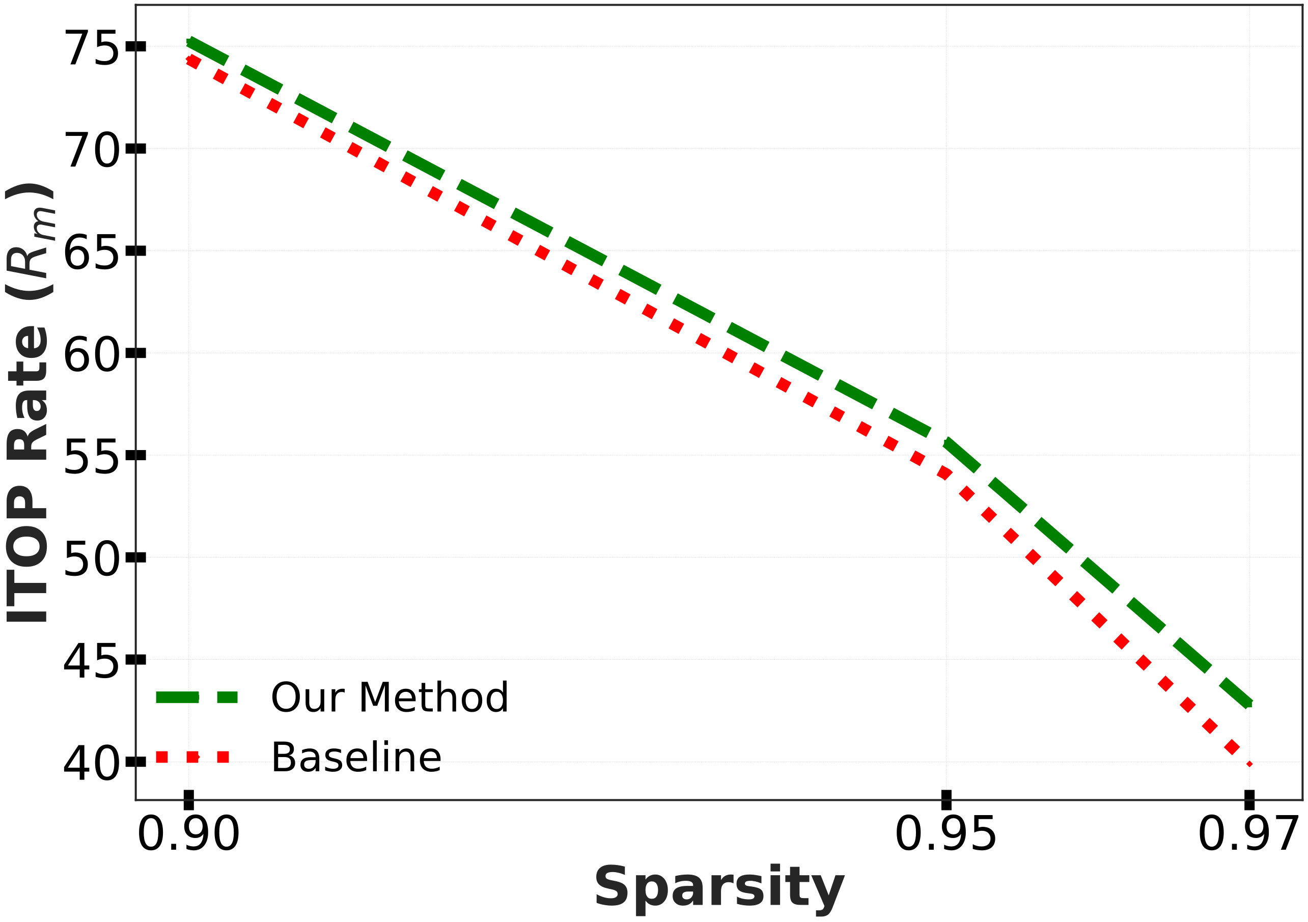
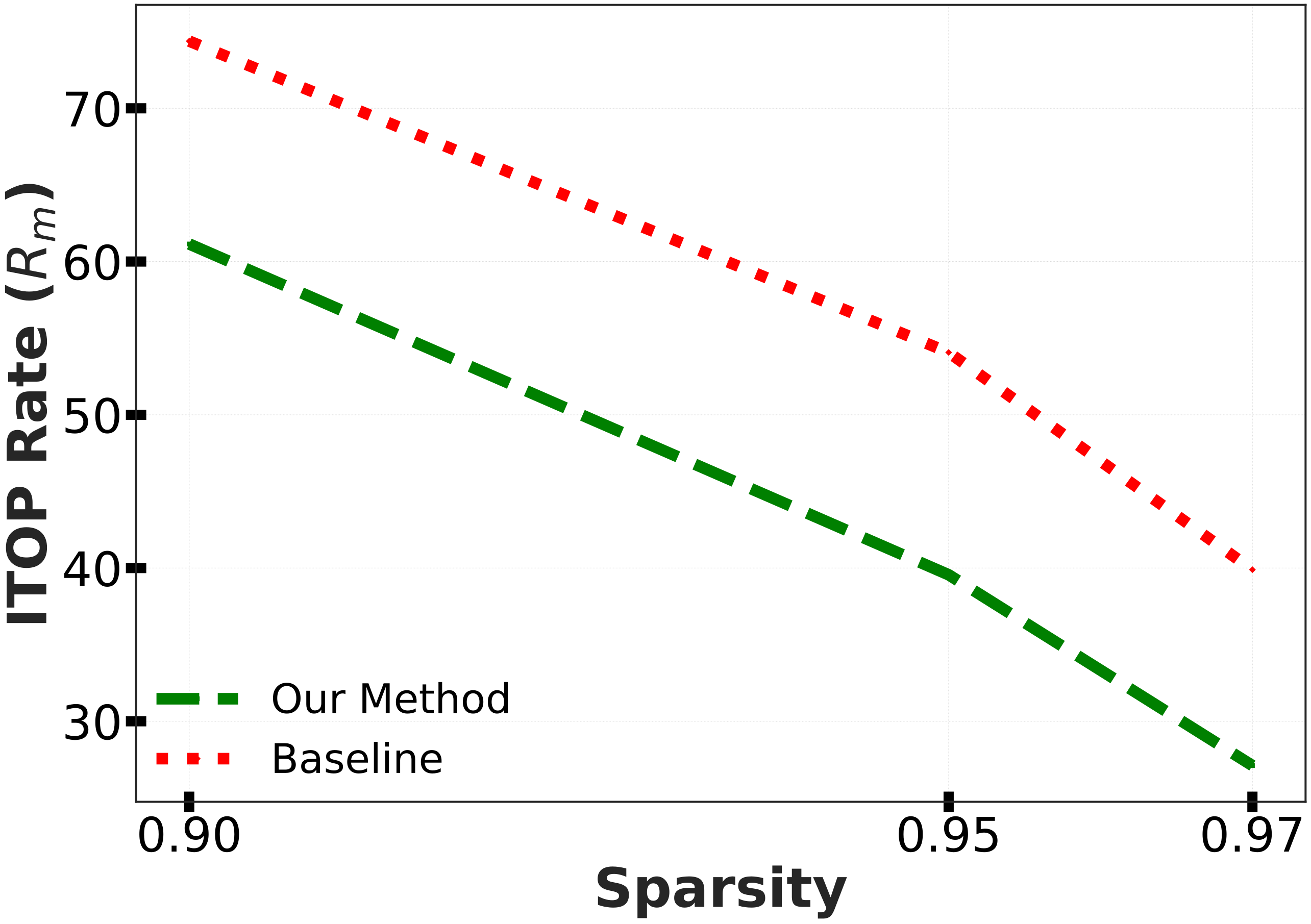
However, using the corrected gradients for mask exploration as well can slightly reduce ITOP in some settings — modifying the gradient ranking changes which connections are prioritized, potentially in ways that reduce diversity. This finding highlights that mask exploration in DST is not independent of optimization: the gradient scaling induced by BN implicitly shapes which sparse topologies are discovered during training.
Compatibility with Other Sparse Optimizers
Recent work has proposed several optimizers specifically designed for sparse training, including HAM (Hyperbolic Aware Minimization)
We show analytically that SparseOpt and HAM address orthogonal aspects of sparse training — SparseOpt corrects BN-induced gradient direction distortion, while HAM encourages implicit sparsification in the outer-layer parameters. We prove this via a balance invariant argument: the BN rescaling and mask changes only affect the gradient flow of the inner-layer weights $w$, and do not disturb the invariant that governs HAM’s sign-flip behavior. Therefore, the two methods can be combined without interference.
Empirically, SparseOpt + HAM consistently outperforms either method alone across all sparsity levels and training schedules on CIFAR-100.
| Sparsity | Method | 100 epochs | 200 epochs | 300 epochs | 500 epochs |
|---|---|---|---|---|---|
| 95% | SparseOpt + HAM (Ours) | $57.31 \pm 0.54$ | $60.41 \pm 0.28$ | $60.91 \pm 0.45$ | $62.20 \pm 0.38$ |
| SparseOpt alone | $56.80 \pm 0.49$ | $59.91 \pm 0.45$ | $60.67 \pm 0.63$ | $61.74 \pm 0.35$ | |
| Baseline (w/ HAM) | $56.72 \pm 0.40$ | $58.76 \pm 0.60$ | $60.38 \pm 0.23$ | $61.66 \pm 0.26$ | |
| Baseline (SGD) | $55.80 \pm 0.73$ | $59.22 \pm 0.55$ | $60.00 \pm 0.54$ | $61.45 \pm 0.65$ |
A Note on Gradient Direction vs. Gradient Magnitude
Our proposed correction modifies both the direction and the magnitude of the gradient. To isolate the contribution of the directional correction, we run an ablation where we additionally apply gradient renormalization (gradient clipping to unit norm) after the SparseOpt correction. This ensures any improvement comes purely from the corrected descent direction, not from any change in step size.
Even with renormalization, SparseOpt consistently outperforms the baseline — confirming that the gradient direction correction is the primary source of improvement. The corrected gradient direction points more accurately toward useful descent directions, enabling faster and more stable convergence.
Extension to Layer Normalization
While this work focuses on Batch Normalization, the same underlying mechanism applies to other normalization layers. In Appendix D of the paper, we derive analytically that Layer Normalization (LN) also amplifies gradients by a factor of $1/\sqrt{1-s}$ under uniform sparsity. This is particularly relevant for transformer-based architectures, where LN is standard and sparse training is increasingly explored (e.g., for mechanistic interpretability in LLMs). Extending SparseOpt to handle LN-induced gradient skew in transformers is an important direction for future work.
Conclusion
This work identifies a previously overlooked source of slow convergence in Dynamic Sparse Training: Batch Normalization. BN’s gradient scaling, which is benign in dense networks, becomes non-uniform and destabilizing in sparse networks due to heterogeneous per-neuron fan-in. In DST, this effect is compounded by periodic mask updates that abruptly change neuron-wise sparsities, causing discontinuous jumps in the effective gradient direction.
Our proposed optimizer, SparseOpt, corrects this distortion with a simple sparsity-aware diagonal preconditioner. The fix is lightweight, composable with existing optimizers, and consistently improves convergence across datasets, architectures, sparsity levels, and DST methods. We hope this work motivates broader attention to sparsity-aware design of training components — normalization, initialization, optimization, and beyond — as a path toward making sparse training practically competitive with dense training.
Key Takeaway: Many building blocks of modern neural network training — including normalization layers — were designed assuming homogeneous (dense) connectivity. When this assumption is violated, as in sparse networks, these components can behave unexpectedly. Rather than blindly applying techniques developed for dense models, sparse training benefits from designs that explicitly account for heterogeneous connectivity.
Read the full paper: For complete mathematical proofs, ablation studies on gradient direction, and further experimental details, check out our ICML 2026 paper on OpenReview.